Mapping the Chesapeake Bay

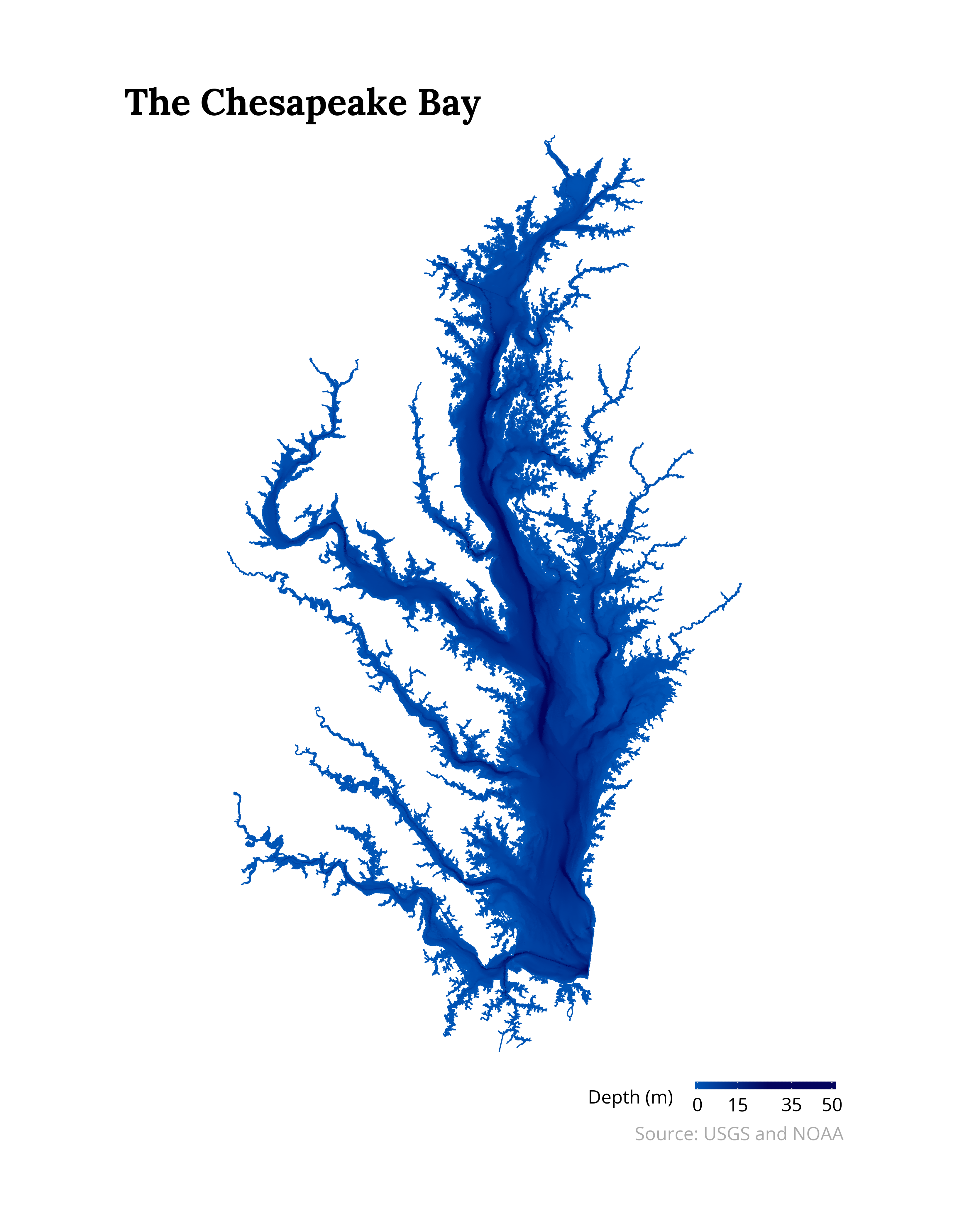
The Chesapeake Bay is the largest estuary in the United States. It is a massive body of water hundreds of miles long and home to a large variety of fish, birds, and of course, crabs! It is also the site of some of the oldest and most historic locations in American history, including Annapolis, Fort McHenry, Jamestown, Williamsburg, Mt. Vernon, the Naval Academy, and more.

I wanted to map the water depths of the Bay as an interdisciplinary exercise spanning ecology, urban/regional planning, cartography, and data science! The plot was generated using USGS (shoreline) and NOAA (water depths) data in Python using geopandas, polars, rasterio, and plotnine! Enjoy the map and code below.

#### Setup ####

import rasterio

import numpy as np
import polars as pl
import plotnine as p9
import geopandas as gp

from rasterio.mask import mask
from pyfonts import load_google_font

DARKBLUE = "#030457"
LIGHTBLUE = "#0066b6"
QUANTILE = 0.99
EXPANSION = 0.42

#### Load Data ####

bay = gp.read_file("P7TidalShorelineDec23.zip")
bay["geometry"] = bay["geometry"].simplify(100)

with rasterio.open("exportImage.tiff") as src:

    # Transform CRS and mask
    bay = bay.to_crs(src.crs)
    out_image, out_transform= mask(src, bay.geometry, crop=True)

    # Create indicies and transform
    rows, cols = out_image[0].shape
    y_indices, x_indices = np.mgrid[0:rows, 0:cols]
    xs, ys = rasterio.transform.xy(out_transform, y_indices, x_indices)

#### Create Plot ####

depth = (
    pl.DataFrame({
        "x": np.array(xs).flatten(),
        "y": np.array(ys).flatten(),
        "depth": 0 - out_image[0].flatten()
    })
    .filter(pl.col("depth") > 0)
    .with_columns(
        # Minor adjustment for plot scale
        pl.col("depth") * 1.05 - 1
    )
)

serif = load_google_font("Lora", weight="bold")
sans = load_google_font("Open Sans")

serif.set_size(30)
sans.set_size(15)

plot = (
    p9.ggplot() +
    p9.geom_point(
        data=depth.sample(n=250_000, seed=42),
        mapping=p9.aes("x", "y", color="depth"),
        size=1e-6
    ) +
    p9.geom_map(
        data=bay,
        color=LIGHTBLUE,
        fill="none"
    ) +
    p9.scale_color_gradient2(
        low=LIGHTBLUE,
        mid=DARKBLUE,
        high=DARKBLUE,
        midpoint=depth.get_column("depth").quantile(QUANTILE),
        breaks=[0, 15, 35, 50]
    ) +
    p9.coord_fixed(
        ratio=1.25
    ) +
    p9.labs(
        color="Depth (m)",
        title="The Chesapeake Bay",
        caption="Source: USGS and NOAA",
    ) +
    p9.expand_limits(
        x=(
            depth.get_column("x").min() - EXPANSION,
            depth.get_column("x").max() + EXPANSION
        )
    ) +
    p9.scale_x_continuous(
        expand=(0, 0)
    ) +
    p9.scale_y_continuous(
        expand=(0, 0)
    ) +
    p9.theme(
        plot_margin=0.09,
        legend_key_height=8,
        legend_key_width=150,
        legend_position="bottom",
        plot_title_position="panel",
        legend_justification="right",
        axis_text=p9.element_blank(),
        axis_title=p9.element_blank(),
        panel_grid=p9.element_blank(),
        panel_background=p9.element_blank(),
        axis_ticks_major=p9.element_blank(),
        text=p9.element_text(fontproperties=sans),
        plot_caption=p9.element_text(color="darkgray"),
        plot_title=p9.element_text(fontproperties=serif, ha="left")
    )
)

#### Save Plot ####

plot.save(
    filename="chesapeake-depth.png",
    height=14,
    width=11,
    dpi=300,
)

Sources

• USGS: Shoreline data comes from P7TidalShorelineDec23.zip
• NOAA: Water depth comes from Coastal Relief Mosaic via the Bathymetric Data Viewer