Estimating Downtown Tree Canopy

Today I am working on using satellite imagery to determine the level of tree canopy coverage in four major east coast downtowns. In particular, I am comparing Atlanta, Charlotte, Washington DC, and Philadelphia. This sits at the intersection of two of my favorite domains; urban planning and data science!

Methods

I chose a superpixel segmentation approach paired with a Gradient Boosting Classifier because pixel-level classifications often suffer from extreme “salt-and-pepper” noise in high-resolution satellite imagery. By grouping contextually similar pixels into cohesive geographic segments, the model evaluates structural shape and localized color variances simultaneously. This allows me to label a handful of segmente per city, build a model, and estimate tree coverage on the remaining segments.

Setup

First, let’s begin with imports, script parameters, and helper functions:

import random

import numpy as np
import polars as pl
import plotnine as p9
import contextily as cx
import matplotlib.pyplot as plt

from sklearn.model_selection import RandomizedSearchCV
from skimage.segmentation import slic, mark_boundaries
from sklearn.ensemble import GradientBoostingClassifier

ZOOM = 16
N_SEGMENTS = 5_000
COMPACTNESS = 0.001
LABELS_PER_CITY = 50
GREEN_THRESHOLD = 0.25
TREE_SAMPLE = 15_000

random.seed(42)
np.random.seed(42)

CITY_HALLS_MERCATOR = {
    "Atlanta": [-9394119, 3993616, -9391119, 3996616],
    "Charlotte": [-9000835, 4195865, -8997835, 4198865],
    "Washington DC": [-8575940, 4704635, -8572940, 4707635],
    "Philadelphia": [-8368832, 4857540, -8365832, 4860540]
}


def show_segment_boundaries(city, path, images, segments):
    boundaries = mark_boundaries(
        images[city],
        segments[city],
        color=(1, 0, 0, 1),
        outline_color=(1, 0, 0, 1),
        mode="thick"
    )
    
    plt.imshow(boundaries)
    plt.axis("off")
    plt.savefig(path)
    plt.close()


def show_segment(city, images, segments, idx):
    segment = segments[city]
    image = images[city]

    coords = np.argwhere(segment == idx)
    mask = image * (segment == idx)[..., np.newaxis]
    
    y_min, x_min = coords.min(axis=0)
    y_max, x_max = coords.max(axis=0)
    
    plt.imshow(mask[y_min:y_max+1, x_min:x_max+1])
    plt.axis("off")
    plt.show()
    plt.close()


def label_trees():
    while True:
        response = input("Is this tree coverage (y/n)? ")
        if response in ["y", "n"]:
            return 1.0 if response == "y" else 0.0
        print("Invalid input. Please enter 'y' or 'n'.")


def get_features(city, images, segments, idx):
    segment = segments[city]
    image = images[city]
    pixels = image[segment == idx]

    return {
        "city": city,
        "idx": idx,
        "mean_r": np.mean(pixels[:, 0]),
        "mean_g": np.mean(pixels[:, 1]),
        "mean_b": np.mean(pixels[:, 2]),
        "std_r": np.std(pixels[:, 0]),
        "std_g": np.std(pixels[:, 1]),
        "std_b": np.std(pixels[:, 2]),
        "segment_size": len(pixels)
    }


def rgb_to_hex(color):
    return f"#{color[0]:02x}{color[1]:02x}{color[2]:02x}"

Satellite Imagery

Next, we can collect satellite images using contextily imported as cx. This utility pulls Esri images using Mercator coordinates at a specific zoom level. The Mercator coordinates I am using are the approximate locations of each city hall for the four cities in my study.

provider = cx.providers.Esri.WorldImagery

images = {
    city: cx.bounds2img(*coords, zoom=ZOOM, source=provider)[0]
    for city, coords in CITY_HALLS_MERCATOR.items()
}

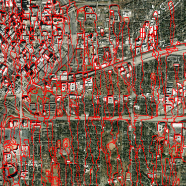
Segmentation

Now we begin the process of segmentation. We will be using slic() from skimage. SLIC (simple linear image clustering) is a common technique to subdivide images into superpixels. Once segmented, we will hand label a few dozen of segments as trees or not trees and then build a model to predict the remainder of the thousands of segments. In the image below, you can see the bounds of the Atlanta segments.

segments = {
    city: slic(image, n_segments=N_SEGMENTS, compactness=COMPACTNESS)
    for city, image in images.items()
}

show_segment_boundaries("Atlanta", "slic-bounds-atlanta.png", images, segments)

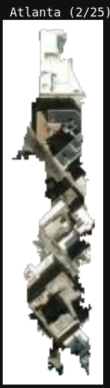
Labelled Data

Next, we set up a pipeline to hand-label a number of segments from each city. In particular, we are labeling 50 images from each city for a total of 200 labeled images. Then we will predict whether the remaining thousands of segments are trees.

While this dataset is fundamentally a small supervised subset paired with a larger unlabeled pool, treating it with a standard classifier over manual annotations operates on a semi-supervised philosophy. This strategy yields far better localized results than a completely unsupervised clustering method.

labels = []
    
for city in CITY_HALLS_MERCATOR.keys():
    unique_segments = np.unique(segments[city])
    sampled_segments = random.sample(list(unique_segments), k=LABELS_PER_CITY) 
    
    for i, idx in enumerate(sampled_segments):
        print(f"{city} ({i + 1}/{LABELS_PER_CITY})")
        show_segment(city, images, segments, idx)
        labels.append({"city": city, "idx": idx, "label": label_trees()})

Here is an example segment from Atlanta:

Model Estimation

Once labelled, we build a dataset of the predicted remaining segments to estimate tree coverage. We are using a mixture of polars and plotnine for modern plotting and dataframe operations.

features = [
    get_features(city, images, segments, idx)
    for city, idxs in segments.items()
    for idx in np.unique(idxs)
]

model_data = (
    pl.DataFrame(features)
    .join(
        other=pl.DataFrame(labels),
        on=["city", "idx"],
        how="left"
    )
)

feature_cols = [
    "mean_r",
    "mean_g",
    "mean_b",
    "std_r",
    "std_g",
    "std_b",
    "segment_size"
]

train = model_data.drop_nulls("label")
design_matrix = model_data.select(feature_cols)

grid = {
    "n_estimators": [100, 200, 300],
    "learning_rate": [0.05, 0.1],
    "max_depth": [3, 5, 10, 15]
}

search = (
    RandomizedSearchCV(
        estimator=GradientBoostingClassifier(),
        param_distributions=grid,
        random_state=42,
        n_iter=3,
        cv=3
    )
    .fit(
        train.select(feature_cols).to_numpy(), 
        train.get_column("label").to_numpy()
    )
)

model = search.best_estimator_

predictions = (
    model_data
    .with_columns(
        trees = model.predict_proba(design_matrix)[:, 1]
    )
    .select("city", "idx", "trees")
)

segment_data = []

for city, segment in segments.items():
    for row_id, contents in enumerate(segment):
        for col_id, idx in enumerate(contents):
            color = images[city][row_id, col_id]
            segment_data.append({
                "city": city,
                "row_id": row_id,
                "col_id": col_id,
                "idx": idx,
                "color": rgb_to_hex(color)
            })
    
plotting_data = (
    pl.DataFrame(segment_data)
    .join(
        other=predictions,
        on=["city", "idx"],
        how="left"
    )
    .with_columns(
        (0 - pl.col("row_id")).alias("row_id")
    )
)

print(
    plotting_data
    .group_by("city")
    .agg(
        pl.col("trees").mean()
    )
)

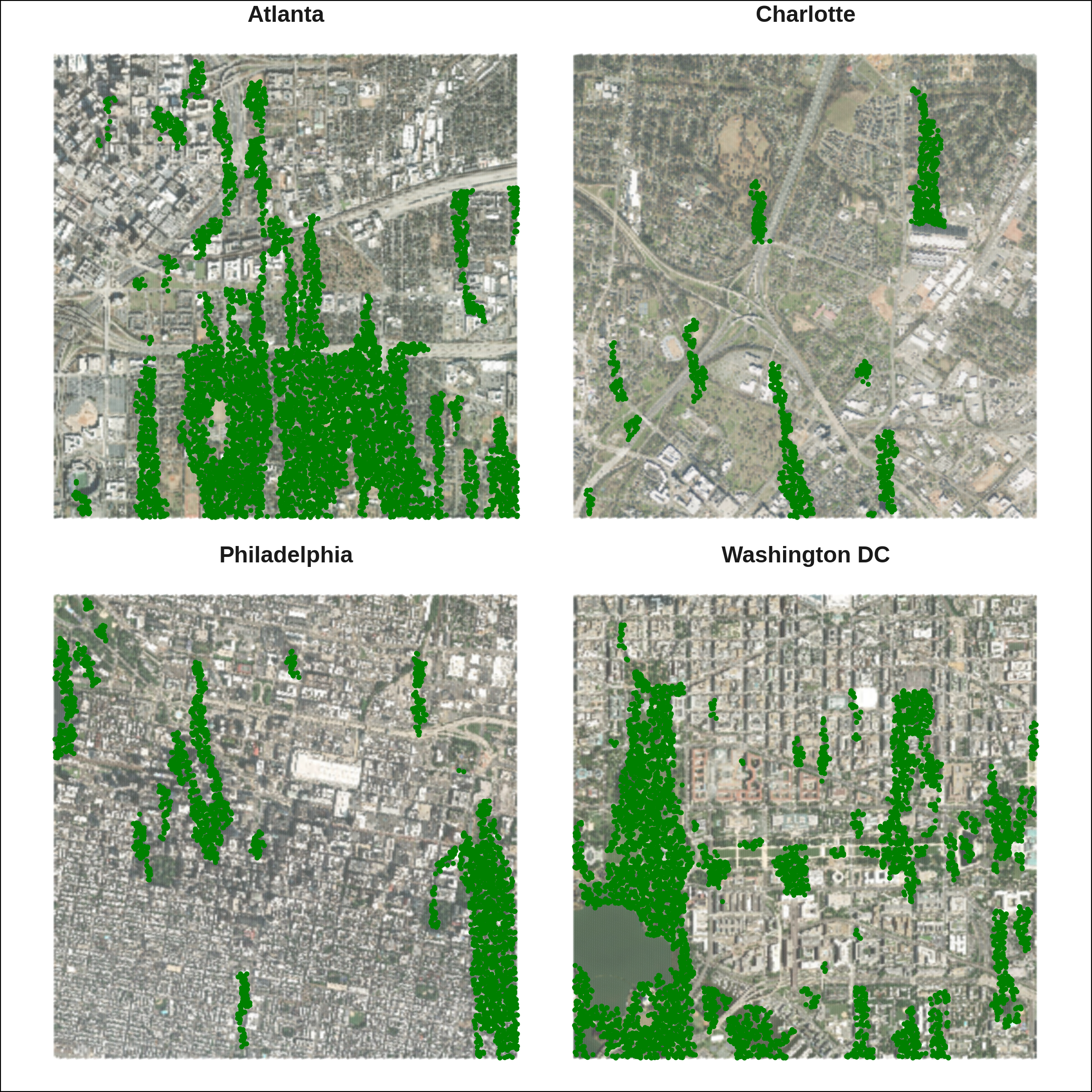
Results

And here is the final plot! You can see the plotnine code below the image shown here. Using a simple percent of pixels predicted to be trees we estimate the following canopy levels for each downtown core:

City	Percent Tree Canopy
Atlanta	19%
Charlotte	12%
Philadelphia	10%
Washington DC	16%

plot = (
    p9.ggplot(
        data=(
            plotting_data
            .filter(pl.col("trees") > GREEN_THRESHOLD)
            .sample(n=TREE_SAMPLE, seed=42)
        ),
        mapping=p9.aes(x="col_id", y="row_id")
    ) +
    p9.geom_point(
        data=(
            plotting_data
            .with_row_index("row")
            .filter(
                (pl.col("row") % 30) == 0
            )
        ),
        mapping=p9.aes(color="color"),
        alpha=0.25,
        size=1e-4
    ) +
    p9.geom_point(
        color="green",
        size=0.5
    ) +
    p9.facet_wrap("city") +
    p9.theme_minimal() +
    p9.coord_fixed() +
    p9.scale_color_identity() +
    p9.theme(
        axis_text=p9.element_blank(),
        panel_grid=p9.element_blank(),
        axis_title=p9.element_blank(),
        text=p9.element_text(size=12, face="bold")
    )
)

plot.save(
    filename="canopy-plot.png", 
    width=8, 
    height=8, 
    dpi=300
)

Comparative Context

Our downtown canopy estimates (10% for Philadelphia to 19% for Atlanta) align well with external urban studies (Maco, n.d.), which typically place dense commercial cores between 8% and 15% coverage. However, these numbers are vastly lower than city-wide municipal assessments. For example, Atlanta boasts a 46% overall canopy rate, highlighting the severe green infrastructure deficit when isolating impervious downtown centers.

In the future we could also work to distinguish contiguous tree canopy from single-family home (SFH) neighborhoods is a major hurdle. These zones often feature lawns, ornamental shrubs, and individual trees that trick models into overestimating canopy density without providing the actual ecological benefits of a dense, unified forest structure.

References

Maco, S. E. (n.d.). Assessing canopy cover over streets and sidewalks in street tree populations. Journal of Arboriculture, 28(6), 270–276.