Building a Stock Market Agent

I wanted to see if I could build a stock market agent leveraging open source models, ollama, Python, and real stock market data. The agent should accept a persona in plain-text which describes it trading strategy. The agent will begin with a fixed amount of cash which it can use to buy and sell three different stocks:

Risk Level	Stock Ticker	Rationale
Low Risk	VOO	A broad market indicator considered safe
Medium Risk	NVDA	A high performance, but somewhat risky tech stock
High Risk	SMCI	An extremely volatile tech stock

At each turn (representing one week of trading) I take the closing price of each of these stocks and allow the agent to buy, sell, or hold its position based on new market data. It also has history of recent trades and current market prices.

This leverages pydantic and structured output to validate the JSON output. It ensures the LLM responds using only a valid set of possible responses using the BaseModel.

import tqdm
import ollama
import yfinance

import polars as pl
import plotnine as p9

from typing import Literal
from pydantic import BaseModel, Field

MODEL = "llama3.2"
MIN_DATE = "2025-01-01"
MAX_DATE = "2026-03-31"

#### Prepare Stock Data ####

market_data = (
    yfinance.download(
        tickers=["VOO", "NVDA", "SMCI"],
        start=MIN_DATE,
        end=MAX_DATE,
        progress=False,
        interval="1wk"
    )
    .get("Close")
    .reset_index()
    .pipe(pl.DataFrame)
    .sort("Date")
    .select(
        pl.col("Date").dt.to_string("%Y-%m-%d").alias("date"),
        pl.col("VOO").round(2).alias("LOW_RISK"),
        pl.col("NVDA").round(2).alias("MED_RISK"),
        pl.col("SMCI").round(2).alias("HIGH_RISK"),
    )
    .iter_rows(
        named=True
    )
)

#### Define Agent Behavior ####

class Decision(BaseModel):
    ticker: Literal["LOW_RISK", "MED_RISK", "HIGH_RISK"]
    action: Literal["BUY", "SELL", "HOLD"]
    quantity: int = Field(description="Must be 0 if holding.")

class Agent:
    def __init__(self, persona: str):
        self.persona = persona
        self.cash = 10000.0
        self.shares = {"LOW_RISK": 0, "MED_RISK": 0, "HIGH_RISK": 0}
        self.history = []
        self.portfolio_value = []

    def advance(self, stock_prices: dict):
        # We only feed the last 3 logs to keep context window overhead minimal
        prompt = f"""
        Output your next trading decision. Maximize
        the value of your portfolio. 
        
        Strategy: {self.persona}
        Balances: Cash ${self.cash:.2f} | Shares {self.shares}
        Market Prices: { {k: v for k, v in stock_prices.items() if k != 'date'} }
        Recent Actions: {self.history[-3:]}
        """

        response = ollama.chat(
            model=MODEL,
            messages=[{"role": "user", "content": prompt}],
            format=Decision.model_json_schema()
        )

        order = Decision.model_validate_json(response.message.content)
        price = stock_prices[order.ticker]

        if order.action == "BUY" and self.cash >= order.quantity * price:
            self.cash -= order.quantity * price
            self.shares[order.ticker] += order.quantity
            self.history.append(f"{stock_prices}: Bought {order.quantity} {order.ticker}")
        elif order.action == "SELL" and self.shares[order.ticker] >= order.quantity:
            self.shares[order.ticker] -= order.quantity
            self.cash += order.quantity * price
            self.history.append(f"{stock_prices}: Sold {order.quantity} {order.ticker}")
        else:
            self.history.append(f"{stock_prices}: Held positions")

        # Portfolio total value calculation (Cash + Asset Value)
        asset_value = sum(self.shares[i] * stock_prices[i] for i in self.shares)
        self.portfolio_value.append(round(self.cash + asset_value, 2))

Next we run the simulation! I ran this over a 1.25 year period starting in 2025 Q1 and ending in 2026 Q1. You can see the three personas defined here:

agents = {
    "Conservative": Agent("Holds low risk stocks over long periods and does not trade often"),
    "Active": Agent("A modest investor who occasionally trades"),
    "Aggressive": Agent("A high risk investor who makes frequent trades")
}

for stock_prices in tqdm.tqdm(market_data):
    for label, agent in agents.items():
        agent.advance(stock_prices)

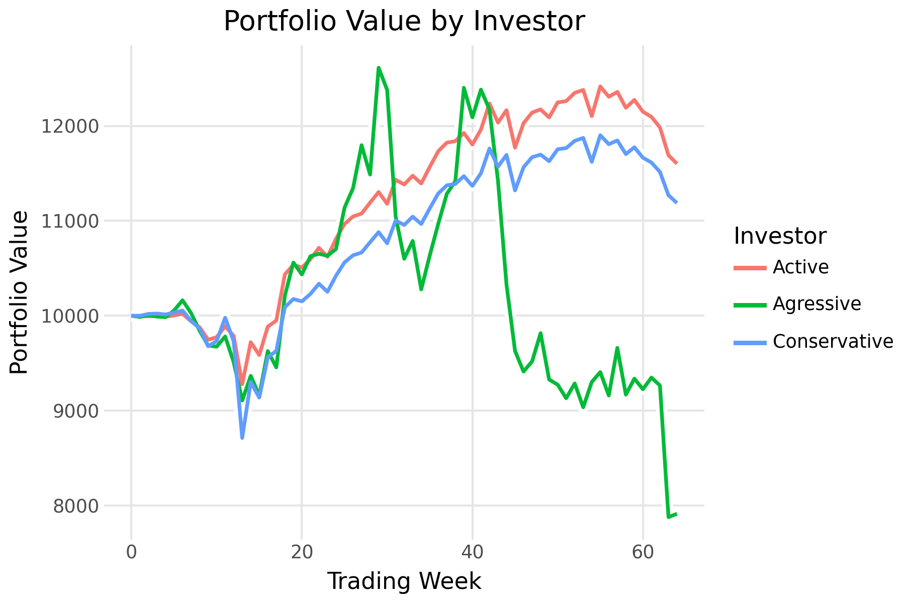
Finally, we visualize the results. We can see that the conservative agent made few trades generally holding VOO throughout the simulation. The medium-risk agent made a few more trades and the high-risk agent traded often!

The conservative agent performed only slightly worse than the moderate agent. Meanwhile, the aggressive agent made significant gains before losing their portfolio during market volatility.

results = (
    pl.DataFrame({
        k: v.portfolio_value
        for k, v in agents.items()
    })
    .with_row_index("day")
    .unpivot(
        index="day"
    )
)

plot = (
    p9.ggplot(
        data=results,
        mapping=p9.aes(
            x="day",
            y="value",
            color="variable",
            group="variable"
        )
    ) +
    p9.geom_line(
        size=3,
        color="white"
    ) +
    p9.geom_line(
        size=1
    ) +
    p9.theme_minimal() +
    p9.theme(
        panel_grid_minor=p9.element_blank()
    ) +
    p9.labs(
        x="Trading Week",
        y="Portfolio Value",
        title="Portfolio Value by Investor",
        color="Investor"
    )
)

Future enhancements include:

• Introducing cash flows (simulating a salary) so agents can distribute new cash
• Introducing more stock tickers
• Introducing qualitative information (headlines, world events)